Efficient Frontier without Risk-Free Asset

With the solution to the mean-variance optimization problem in hand, we can, for any target expected return $E[\tilde r_p]$, determine the optimal weights $\boldsymbol W^*$, as well as the corresponding variance $\sigma^2_p$ and expected return $E[\tilde r_p]$. This allows us to explore three core features of mean-variance optimization:

• The weight vector $\boldsymbol W^*$ for different target expected returns $E[\tilde r_p]$ (Two Fund Theorem)
• The relationship between expected return $E[\tilde r_p]$ and variance $\sigma^2_p$ (Efficient Frontier)
• Covariance properties (e.g., with the minimum variance portfolio (MVP), zero covariance portfolios, etc.)

Let’s examine each in turn.

Two Fund Theorem

From the previous section, the optimal weight vector $\boldsymbol W^*$ for a given target expected return $E[\tilde r_p]$ is:

\[\boldsymbol W^* = \boldsymbol g + \boldsymbol h \cdot E[\tilde r_p],\]

where:

• $\boldsymbol g = \frac{1}{D} \left( B \cdot \boldsymbol V^{-1} \boldsymbol 1 - A \cdot \boldsymbol V^{-1} \boldsymbol \mu \right)$
• $\boldsymbol h = \frac{1}{D} \left( C \cdot \boldsymbol V^{-1} \boldsymbol \mu - A \cdot \boldsymbol V^{-1} \boldsymbol 1 \right)$

All optimal weights are linear functions of the target expected return $E[\tilde r_p]$. As $E[\tilde r_p]$ varies, so does the optimal weight vector, but all such vectors lie on a straight line in $\mathbb{R}^N$ (the weight space). This means any two optimal portfolios can be combined to construct any other optimal portfolio—a result known as the Two Fund Theorem.

Claim:

For any two optimal portfolios, any linear combination of them is also an optimal portfolio:

\[\boldsymbol W^* = \alpha \boldsymbol W^*_1 + (1 - \alpha) \boldsymbol W^*_2, \quad \forall \alpha \in [0, 1]\]

Proof:

Since both are optimal portfolios, we can write:

\[\begin{align*} \boldsymbol W^*_1 = \boldsymbol g_1 + \boldsymbol h_1 \cdot E[\tilde r_1], \\ \boldsymbol W^*_2 = \boldsymbol g_2 + \boldsymbol h_2 \cdot E[\tilde r_2], \end{align*}\]

where $\boldsymbol g_1, \boldsymbol h_1$ and $\boldsymbol g_2, \boldsymbol h_2$ are the optimal weights for portfolios 1 and 2, respectively. The linear combination is:

\[\begin{align*} \boldsymbol W^* &= \alpha \boldsymbol W^*_1 + (1 - \alpha) \boldsymbol W^*_2 \\ &= \alpha (\boldsymbol g_1 + \boldsymbol h_1 E[\tilde r_1]) + (1 - \alpha)(\boldsymbol g_2 + \boldsymbol h_2 E[\tilde r_2]) \\ &= \alpha \boldsymbol g_1 + (1 - \alpha) \boldsymbol g_2 + \alpha \boldsymbol h_1 E[\tilde r_1] + (1 - \alpha) \boldsymbol h_2 E[\tilde r_2] \\ &= \boldsymbol g + \boldsymbol h E[\tilde r_p] \end{align*}\]

where:

• $\boldsymbol g = \alpha \boldsymbol g_1 + (1 - \alpha) \boldsymbol g_2$
• $\boldsymbol h = \alpha \boldsymbol h_1 + (1 - \alpha) \boldsymbol h_2$
• $E[\tilde r_p] = \alpha E[\tilde r_1] + (1 - \alpha) E[\tilde r_2]$

Thus, any linear combination of two optimal portfolios is also optimal. This is the Two Fund Theorem.

Note: Optimal portfolios are also called frontier portfolios (see the Efficient Frontier section below).

Efficient Frontier (Without Risk-Free Asset)

Since $\boldsymbol W^*$ traces a straight line in weight space, what does this look like in mean-variance space ($\mu, \sigma^2$) or mean-standard deviation space ($\mu, \sigma$)?

Recall that $\boldsymbol W^*$ is a linear function of $E[\tilde r_p]$, and the portfolio variance $\sigma^2_p = \boldsymbol W_p^T V \boldsymbol W_p$. The relationship between $E[\tilde r_p]$ and $\sigma^2_p$ is:

\[\begin{align*} \sigma^2_p &= \boldsymbol W^T \boldsymbol V \boldsymbol W \\ &= (\boldsymbol g + \boldsymbol h E[\tilde r_p])^T \boldsymbol V (\boldsymbol g + \boldsymbol h E[\tilde r_p]) \\ &= \frac{C}{D} [E(\tilde r_p) - \frac{A}{C}]^2 + \frac{1}{C} \end{align*}\]

Thus, $\sigma^2_p$ is a quadratic function of $E[\tilde r_p]$. Plotting expected return against variance yields a hyperbola. The minimum variance portfolio (MVP) is the point on the hyperbola with the lowest variance.

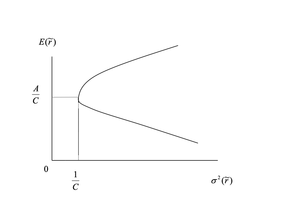
Minimum Variance Portfolio (MVP)

The MVP is the point on the hyperbola with minimum variance. It has expected return $E[\tilde r_{mvp}] = \frac{A}{C}$ and variance $\sigma^2_{mvp} = \frac{1}{C}$.

Efficient Frontier

According to utility theory, if only the mean and variance of wealth matter, any rational investor would choose the portfolio with the highest expected return for a given level of variance (the top left of the mean-variance space). Thus, only the upper half of the hyperbola is desirable—the efficient frontier. In summary:

• Frontier Portfolios
  • All points on the hyperbola are frontier portfolios
  • Each is the lowest variance portfolio for a given expected return
  • The frontier is the edge of all feasible portfolios
  • Any two frontier portfolios can be combined to form another frontier portfolio
• Minimum Variance Portfolio (MVP)
  • The pivot point of the hyperbola
  • The MVP is the lowest variance portfolio of all portfolios
• Efficient Frontier
  • The upper half of the hyperbola
  • Corresponds to $E(\tilde r_p) > E(\tilde r_{mvp}) = \frac{A}{C}$
• Inefficient Portfolios
  • The lower half of the hyperbola
  • Corresponds to $E(\tilde r_p) < E(\tilde r_{mvp}) = \frac{A}{C}$
  • Not desirable

Mean-Standard Deviation Space

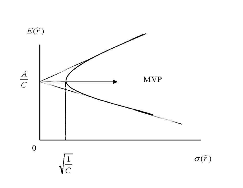
The asymptotes are given by:

\[E[\tilde r_p] = \frac{A}{C} + \sqrt{\frac{D}{C}} \cdot \sigma_p\]

Covariance Properties

Covariance Between Portfolios

The covariance between any two portfolios can be calculated using the covariance matrix $V$:

\[Cov(\tilde r_p, \tilde r_q) = \boldsymbol W_p^T \boldsymbol V \boldsymbol W_q\]

where $\boldsymbol W_p$ and $\boldsymbol W_q$ are the weight vectors of the two portfolios.

Covariance of Frontier Portfolios

Recall the variance of a frontier portfolio:

\[\sigma^2_p = \frac{C}{D} [E(\tilde r_p) - \frac{A}{C}]^2 + \frac{1}{C}\]

Similarly, the covariance between any two frontier portfolios is:

\[Cov(\tilde r_p, \tilde r_q) = \frac{C}{D} [E(\tilde r_p) - \frac{A}{C}] [E(\tilde r_q) - \frac{A}{C}] + \frac{1}{C}\]

Covariance with the Minimum Variance Portfolio (MVP)

Claim:

The covariance between any portfolio (not necessarily a frontier portfolio) and the MVP is equal to the variance of the MVP:

\[Cov(\tilde r_p, \tilde r_{mvp}) = \sigma^2_{mvp}\]

Proof:

Consider the portfolio $\alpha \tilde r_p + (1 - \alpha) \tilde r_{mvp}$, where $\alpha$ is a constant. The variance is:

\[\begin{align*} Var(\alpha \tilde r_p + (1 - \alpha) \tilde r_{mvp}) &= \alpha^2 Var(\tilde r_p) + (1 - \alpha)^2 Var(\tilde r_{mvp}) + 2\alpha(1 - \alpha) Cov(\tilde r_p, \tilde r_{mvp}) \\ &= \alpha^2 \sigma^2_p + (1 - \alpha)^2 \sigma^2_{mvp} + 2\alpha(1 - \alpha) Cov(\tilde r_p, \tilde r_{mvp}) \end{align*}\]

The minimum variance is achieved at $\alpha = 0$ (since the MVP is the lowest variance portfolio). The first-order condition (FOC) is:

\[\begin{align*} \frac{\partial Var(\alpha \tilde r_p + (1 - \alpha) \tilde r_{mvp})}{\partial \alpha} &= 2\alpha \sigma^2_p + 2(1 - \alpha) \sigma^2_{mvp} + 2\alpha Cov(\tilde r_p, \tilde r_{mvp}) - 2(1 - \alpha) Cov(\tilde r_p, \tilde r_{mvp}) = 0 \end{align*}\]

Plugging in $\alpha = 0$:

\[\begin{align*} 2 \sigma^2_{mvp} - 2 Cov(\tilde r_p, \tilde r_{mvp}) = 0 \\ Cov(\tilde r_p, \tilde r_{mvp}) = \sigma^2_{mvp} \end{align*}\]

Thus, the covariance between any portfolio and the MVP equals the variance of the MVP.

Zero Covariance Portfolio

Claim:

For any frontier portfolio $p$ (except the MVP), there exists a unique frontier portfolio $zc(p)$ such that the covariance between $p$ and $zc(p)$ is zero.

Proof:

Set

\[Cov(\tilde r_p, \tilde r_q) = \boldsymbol W_p^T \boldsymbol V \boldsymbol W_q\]

where $\boldsymbol W_p$ and $\boldsymbol W_q$ are the weights of portfolios $p$ and $q$. Using the definitions of $\lambda$ and $\gamma$ for $p$:

\[\begin{align*} \lambda &= \frac{C E[\tilde r_p] - A}{D} \\ \gamma &= \frac{B - A E[\tilde r_p]}{D} \end{align*}\]

We can show:

\[E[\tilde r_q] = E[\tilde r_{zc(p)}] + \frac{Cov(\tilde r_p, \tilde r_q)}{\sigma^2_{p}} \{E[\tilde r_p] - E[\tilde r_{zc(p)}]\}\]

where $\beta_{qp} = \frac{Cov(\tilde r_p, \tilde r_q)}{\sigma^2_{p}}$ is the beta of portfolio $q$ with respect to $p$.

Interpretation:

Any portfolio $q$ (not the MVP) can be expressed, explained, or constructed from a frontier portfolio $p$ and its zero covariance portfolio $zc(p)$.

This provides a new perspective for explaining expected returns. In the mean-variance framework, we relate expected return to variance. Now, we can also relate expected return to $\beta_{qp}$: higher beta implies higher expected return.

Later, we will introduce the Market Portfolio, a special case where substituting the market portfolio for $p$ yields the Security Market Line (SML), which leads to the Capital Asset Pricing Model (CAPM). This will be discussed in the next section.

Conclusion

Key takeaways from this section:

• The optimal weights $\boldsymbol W^*$ are linear functions of the target expected return $E[\tilde r_p]$.
• The portfolio variance $\sigma^2_p$ is a quadratic function of $E[\tilde r_p]$.
• The minimum variance portfolio (MVP) is the point on the hyperbola with the lowest variance.
• The efficient frontier is the upper half of the hyperbola; the lower half is inefficient.
• The covariance between any portfolio and the MVP equals the variance of the MVP.
• The covariance between any two frontier portfolios is given by the covariance matrix $V$.
• For any frontier portfolio $p$ (except the MVP), there exists a unique frontier portfolio $zc(p)$ with zero covariance with $p$.
• Any portfolio $q$ (not the MVP) can be expressed or constructed from a frontier portfolio $p$ and its zero covariance portfolio $zc(p)$.