Frontier With Risk-Free Asset

Now we introduce the risk-free asset into the mean-variance analysis. The risk-free asset is an asset that has a certain return and no risk, we normally use the return of treasury bills as the risk-free rate. The risk-free asset is a theoretical concept, but it is a useful tool in finance. The risk-free asset has the following properties:

1. The return of the risk-free asset is known with certainty, $r_f$.
2. The risk-free asset has no risk, meaning the variance of the return is zero, $\sigma_{r_f}^2 = 0$.
3. Zero covariance with all risky assets, $Cov(r_f, r_i) = 0$.

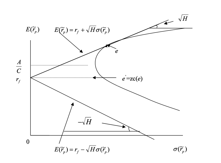
Thus, the combination of the risk-free asset with any risky asset will form a straight line in the mean-variance space. Just by intuition, since investors would like to have a higher return for a given level of variance (top-left corner in mean-variance space), the tangent line (if exists) from the risk-free asset to the risky frontier hyperbola will be the optimal portfolio, it will form the “new” efficient frontier, show in the figure below:

In the following sections, we will formally derive the equation of the new efficient frontier with the risk-free asset, and show how to find the optimal portfolio.

Optimization Problem with Risk-Free Asset

setup:

• $r_f$: risk-free rate
• $N$: number of risky assets, in total $N+1$ assets (with risk-free asset)
• $W$: $N$-dimensional vector of portfolio weights, only for risky assets
• $W_{rf}$: weight of risk-free asset, $W_{rf} = 1 - \sum_{i=1}^N W_i$
• $\mu$: $N$-dimensional vector of expected returns of risky assets

The problem:

\[\begin{align*} \min_{W} \quad & \frac{1}{2} W^T V W \\ \text{s.t.} \quad & W^T \mu + (1 - W^T \boldsymbol{1}) r_f= E[\tilde r_p] \end{align*}\]

Note: the weight summation constraint is already included.

where $E[\tilde r_p]$ is the expected return of the portfolio, and $\boldsymbol{1}$ is a vector of ones. The first term in the objective function is the variance of the portfolio, and the second term is the expected return of the portfolio. The constraint is that the expected return of the portfolio must be equal to a certain level.

Lagrangian:

\[\mathcal{L}(W, \lambda) = \frac{1}{2} W^T V W + \lambda [E[\tilde r_p] - (W^T \mu + (1 - W^T \boldsymbol{1}) r_f)]\]

The first-order condition is:

\[\begin{align*} \frac{\partial \mathcal{L}}{\partial W} &= V W - \lambda (\mu - r_f \boldsymbol{1}) = 0 \\ \frac{\partial \mathcal{L}}{\partial \lambda} &= E[\tilde r_p] - (W^T \mu + (1 - W^T \boldsymbol{1}) r_f) = 0 \end{align*}\]

That is two equations with two unknowns, $W$ and $\lambda$, solution is:

\[\begin{align*} \lambda &= \frac{E[\tilde r_p] - r_f}{(\mu - r_f \boldsymbol{1})^T V^{-1} (\mu - r_f \boldsymbol{1})} \\ W_p &= \lambda V^{-1} (\mu - r_f \boldsymbol{1}) \\ &= \frac{E[\tilde r_p] - r_f}{(\mu - r_f \boldsymbol{1})^T V^{-1} (\mu - r_f \boldsymbol{1})} V^{-1} (\mu - r_f \boldsymbol{1}) \\ &= V^{-1} (\mu - r_f \boldsymbol{1}) \frac{E[\tilde r_p] - r_f}{H} \end{align*}\]

where $H = (\mu - r_f \boldsymbol{1})^T V^{-1} (\mu - r_f \boldsymbol{1})$.

Mean-Variance relationship of the optimal portfolio and Capital Market Line

With the optimal portfolio $W_p$, we can find the expected return and variance of the portfolio:

\[\begin{align*} \sigma_p^2 &= W_p^T V W_p \\ &= \frac{[E[\tilde r_p] - r_f](\mu - r_f \boldsymbol{1})^T V^{-1} V V^{-1} (\mu - r_f \boldsymbol{1})}{H^2} \\ &= \frac{[E[\tilde r_p] - r_f]^2}{H^2} (\mu - r_f \boldsymbol{1})^T V^{-1} (\mu - r_f \boldsymbol{1}) \\ &= \frac{[E[\tilde r_p] - r_f]^2}{H^2} H \\ &= \frac{[E[\tilde r_p] - r_f]^2}{H} \end{align*}\]

Rearranging the equation, we have:

\[\sigma_p = \begin{cases} \frac{E[\tilde r_p] - r_f}{\sqrt{H}} & \text{if } E[\tilde r_p] > r_f \\ \frac{0}{\sqrt{H}} & \text{if } E[\tilde r_p] = r_f \\ - \frac{E[\tilde r_p] - r_f}{\sqrt{H}} & \text{if } E[\tilde r_p] < r_f \end{cases}\]

That is the figure below:

Again, the frontier above the $r_f$ is the efficient frontier, and the frontier below the $r_f$ is the inefficient frontier. Notice the slope of the line $\sqrt{H} = \frac{E[\tilde r_p] - r_f}{\sigma_p}$, which is the Sharpe ratio of the optimal portfolio, all efficient portfolios have the same Sharpe ratio.

Since all rational investors will only choose the efficient portfolios, we call the line above the $r_f$ the Capital Market Line (CML). The CML is the line that represents the risk-return trade-off of the optimal portfolio with the risk-free asset. The slope of the CML is the Sharpe ratio of the optimal portfolio, which is the same for all efficient portfolios.

Interaction with frontier without risk-free asset

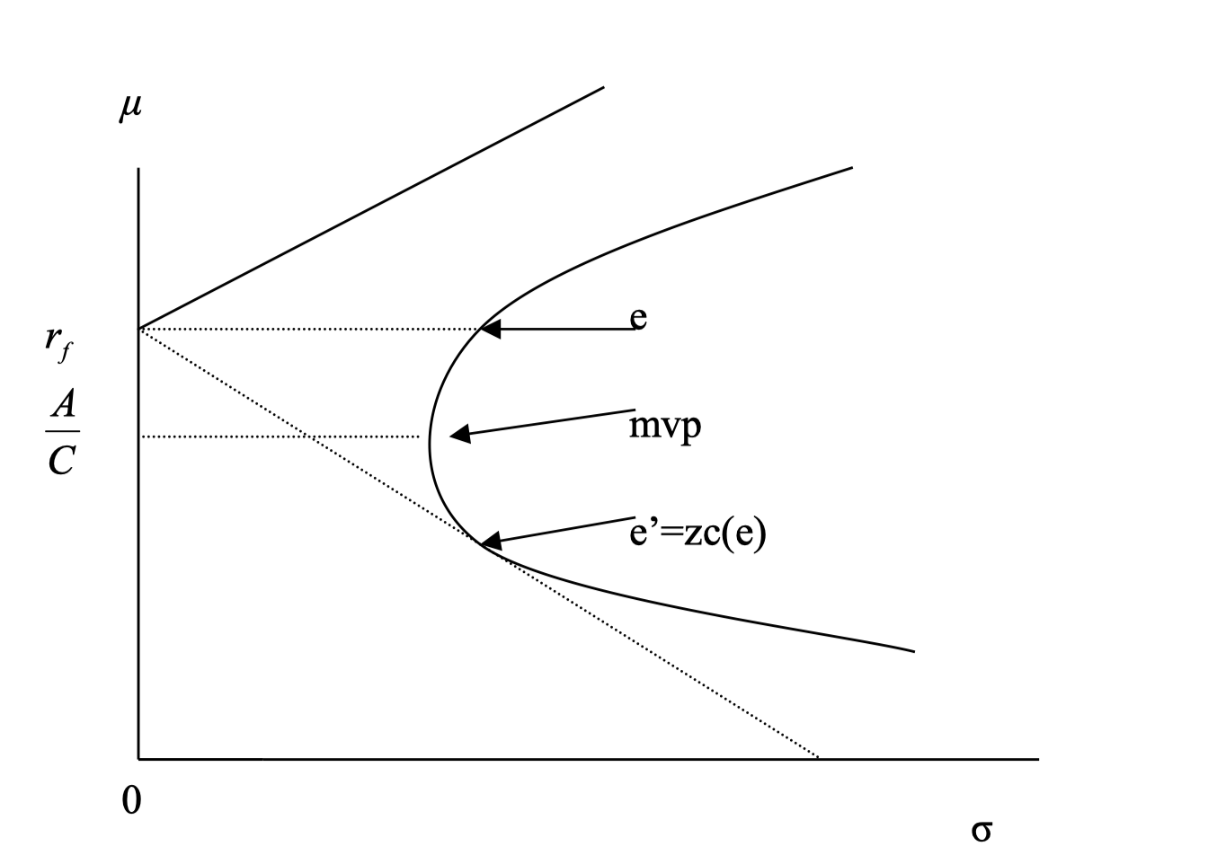
Case 1: $r_f < E[\tilde r_{mvp}] = \frac{A}{C}$

• The efficient frontier would be the tangent line
• Tangent portfolio $e$ is a optimal portfolio with zero risk-free asset
• The efficient frontier above $e$ will require borrowing (negative weight in risk-free asset)
• Zero covariance portfolio $E[\tilde r_{zc(e)}] = r_f$

The tangent portfolio $e$ is really important, it will consider as the “market portfolio” with certain condition, we will discuss this in the next section. Now, let’s figure out the coordinates of the tangent portfolio $e$, by setting the slope of the tangent line equal to partial derivative of the hyperbola on $\sigma$.

The derivative of the hyperbola is:

\[\frac{d E[\tilde r_p]}{d \sigma_p} = \pm \frac{D \sigma_p}{\sqrt{CD\sigma_p^2 - D}}\]

Since $r_f < \frac{A}{C}$, we take the positive sign, set it equal to the slope of the tangent line $\sqrt{H}$, we have:

\[\frac{D \sigma_p}{\sqrt{CD\sigma_p^2 - D}} = \sqrt{H}\]

Solving the equation, we have:

\[\begin{cases} \sigma_p = \sqrt{\frac{H}{CH - D}} \\ E[\tilde r_p] = \frac{A}{C} + \frac{D}{C} \sqrt{\frac{1}{CH - D}} \\ \end{cases}\]

Case 2: $r_f < E[\tilde r_{mvp}] = \frac{A}{C}$

The tangent line will be the in-efficient frontier.

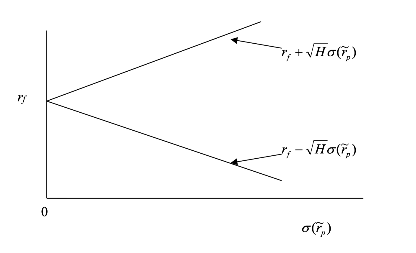
Case 3: $r_f = E[\tilde r_{mvp}] = \frac{A}{C}$

In this case:

\[\begin{align*} H &= B - 2 A r_f + C r_f^2 \\ &= B - 2 A \frac{A}{C} + C \\ &= \frac{BC - A^2}{C} \\ &= \frac{D}{C} \end{align*}\]

Recall the the asymptote of the hyperbola is:

\[\begin{align*} E[\tilde r_p] &= \frac{A}{C} \pm \sqrt{\frac{D}{C}} \sigma_p \\ &= r_f \pm \sqrt{H}\sigma_p \end{align*}\]

Thus, the asymptote is the efficient frontier with risk-free asset, the tangent line is not exist:

Conclusion

Key takeaways:

• The risk-free asset
• The solution to the optimization problem with risk-free asset
• The Capital Market Line (CML)
• The tangent portfolio